Employee Performance and Attrition Analytics

Tuesday. January 07, 2020 - 11 mins

1. Introduction & Business Understanding

Go to this page to download ‘IBM Attrition Dataset’

At any given point in time, about 50% of the employees in an organization are considering changing of employer according to a statistic shared by Gallup. Employee attrition is a huge problem faced by organizations because every outgoing employee takes countless hours of training and other resources invested in him or her by the employer. By understanding what variables in terms of employee characteristics, work experience, etc. increase the probability that an employee would leave the organization, the company can realize significant savings monetary and time wise. This is precisely what we are trying to solve here – find the variables (or predictors) that can influence or determine whether an employee would leave the organization or not. Our project falls under the category of Human Resource (HR) Analytics.

2. Data Description

The dataset is fictional and has been created by IBM data scientists to understand the phenomenon of Attrition. It contains a total of 35 variables in which column ‘Attrition’ is the one we intend to predict. In this case, ‘Attrition’ is our target (or Dependent) variable and the leftover 34 variables, which includes the likes of Gender, Education, Department etc., are predictor (or Independent) variables. ‘Attrition’ is a binary variable, only taking in “Yes” (1) or “No” (0) as values. The total number of rows in the dataset is 1470. Including the column Attrition, there are 21 categorial variables and the rest are continuous in nature. Majority of the categorical variables are encoded in the following manner:

1 = Low 2 = Medium 3 = High 4 = Very High

For education: 1 = Below College 2 = College 3 = Bachelor 4 = Master 5 = Doctor

3. Data Cleaning and Variable Categorization

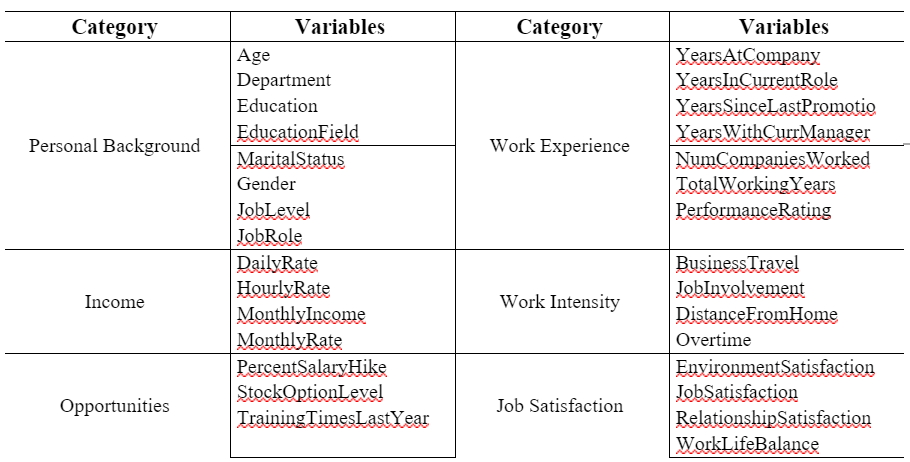
We used the “MICE” package to whether or not there are NULL values in the dataset. The test revealed there are none. After studying the structure, we found 3 columns (‘Over18’, ‘EmployeeCount’, and ‘Standard Hours’) that are constant in nature. These columns were dropped from our analysis. We excluded the column ‘EmployeeNumber’ as well, because it doesn’t add value. Finally, based on the data type of the remaining 30 variables (excluding the target variable), we classify them into 6 categories as listed below:

4. Exploratory Data Analysis

Because our target variable is a categorical one (Yes/No), scatterplots essentially wouldn’t be useful here. Thus, we’ll make judicious use of bar charts, line charts, histograms and mosaic plots to convey our insights.

Now after this you can directly use SQL commands or if you prefer, create new user to use.

1. Attrition Distribution On the Basis of Personal Background

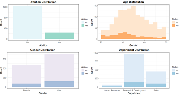
First, we explore the attrition distribution based on personal information. There are 237 employees who left the company, which amounts to 16.1% of the total sample. This quite high as compared to the industry standard of 10% (anything above it is considered problematic).
The age distribution of people who left the company concentrates on people that are between 25-35 years old. As the age goes up, people show less tendency to leave the company. There is no major difference of the attrition distribution between females and males. According to the department distribution, it shows that employees from the R&D and Sales department have higher chances to leave the company.

2. Attrition Distribution on the Basis of Income

Salary is the most (or at least one of the most) motivating factors for an employee. We start our analysis with Monthly Income.

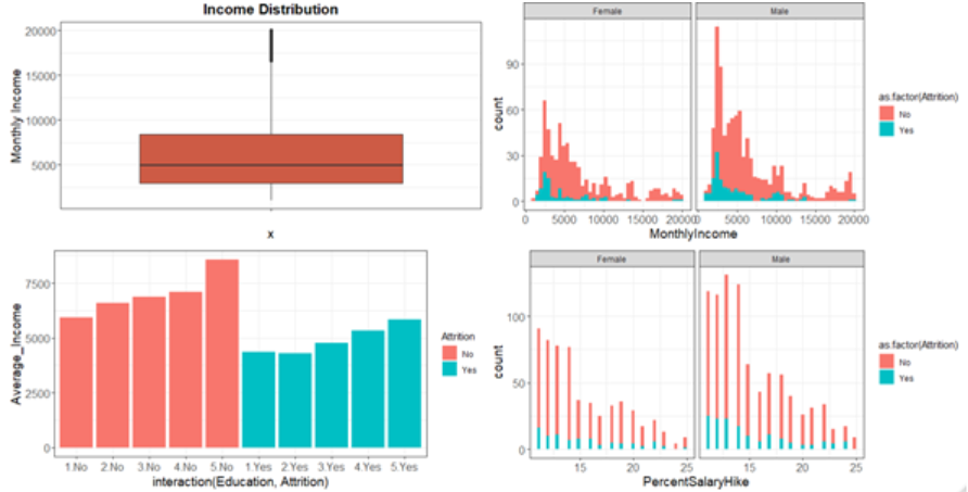
As witnessed from the boxplot, the average monthly income stands at around $6500 and the maximum value goes till $20000. There are some outliers but we’ll keep them untouched as people do earn (or are at least capable of earning) that kind of money.

Next, we further our visualization by plotting a histogram of Monthly income dividing between gender. We suspected that there might be a difference in attrition between male and female when salary is equal, but as evident from the graph, this is clearly not the case. The attrition is highest when the employee is earning in the range of $1000-$7000, which is expected of the range in question.

Moving on, we plotted the interaction of average of Monthly income with level of Education. As suspected, people who left the company had lower average income across all education levels as compared to people who didn’t leave the company. This directly points out to the importance of salary in Attrition.

Next, we investigated % hike and divided that among Male-Female. As witnessed from the graph, lower the % hike, higher is the attrition. But there is no considerable difference in the ratio of Attrition when we differentiate amongst male female which indicates that Gender might not be a strong factor for determining Attrition.

5. Modeling

After running some preliminary visualization analysis, we ran logistic regression on all six categories explained above. One by one, we considered variables in each category alongside ‘Attrition’ as the target variable. We conducted the modelling process on the basis of the six categories mentioned in the beginning; each variable under each category was considered while modelling –

On the Basis of Category ‘Personal Background’

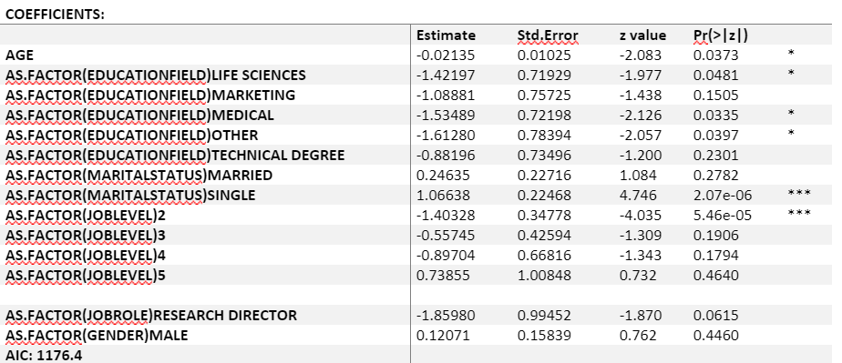
From the result, we can see that age, education field, job level and marital status are significantly correlated with the attrition, and the AIC for this model is 1176.4. Elder people tend to stay in the company. Compared to divorced people, married and single people are prone to leave the company. However, even though ‘Job Role’ is not significantly correlated with attrition, the p-value of ‘Research Director’ is very close to 0.05. If we include ‘Job Role’ and other significant variables and run logistic regression again, the AIC will decrease to 1166.5, lower than excluding it. Therefore, ‘Job Role’ is kept for further analysis.

On the basis of category ‘Income’

We test the correlations among the four variables in this category, and we could not find any significantly strong correlations. (The result is counterintuitive, but this is the fictional data set, and we could not know the algorithm behind hourly, daily, and monthly rate.) Therefore, we include all of them to run the logistic regression.

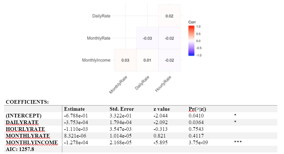
From the result, we can see that only daily rate and monthly rate are significantly correlated with the attrition. For a one-unit increase in the daily rate, the expected change in log odds will decrease by 0.0003753. For a one-unit increase in the monthly income, the expected change in log odds will decrease by 0.0001278. After excluding the insignificant variables, the AIC drops to 1254.6.

On the basis of category ‘Opportunities’

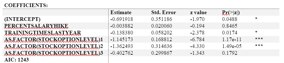
The insignificant variable in this category is % salary hike and stock option level. Then we only include training times last year and stock option level to run a new logistic regression model, we get a lower AIC value of 1241.1. Therefore, we will exclude % salary hike in further analysis.

On the basis of category ‘Work Experience’

Under this category, we explored variables such as Years at Company, Years in Current Role etc.

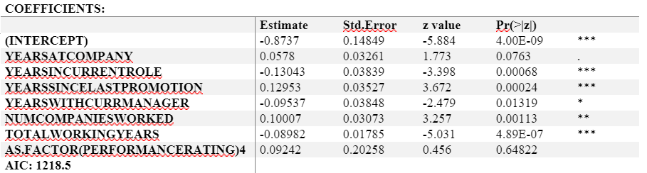
As observable from the results, every variable apart from Performance Rating is significant. People who spend more years at the company are prone to leave the company. Also, a unit increase in Years since last promotion would result in an increase of 0.13 in log odds of Attrition happening, given everything else is held constant.

But an increment in Years in current role would decrease the chances of an employee leaving the organization, which makes sense too. Also a increment in Total Working Years would decrease the log odds of an employee leaving the organization. If we include Performance Rating, we get an AIC of 1218.5 but if we exclude it, we are getting an AIC of 1216.7.

On the basis of category ‘Work Intensity’

We considered variables like Business Travel, Job Involvement etc. in our logit model. The results came out as follows :

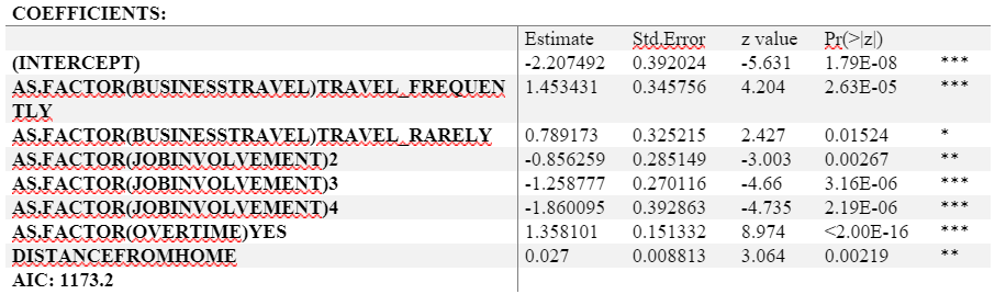
As observable from the results, Employees who travel rarely and frequently are more prone to leave their organizations. The log odds of leaving the organization with regards to a person who travels rarely increases by 0.789 as compared to a person who does not. The log odds increase even more so for an employee who travels frequently which is a comprehendible fact as many employees consider travelling a hassle and would rather have a static job.

Similarly, the log odds of leaving organization with regards to a person working overtime is more as compared to an employee who doesn’t work overtime. Also, as the Distance From Home increases, so does the log odds of a person leaving the company. Finally, the more a person is involved with his/her, the lesser are the log odds of him leaving the company. All these factors are comprehendible.

On the basis of category ‘Job Satisfaction’

We considered variables like Job Satisfaction, Relationship Satisfaction etc. under this category –

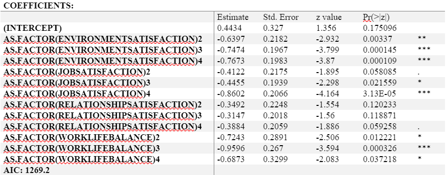
As observable from the results, every variable is significant close to 95% confidence interval except Relationship Satisfaction. People who are more satisfied with their environment and jobs are less likely to change their company and that is abundantly clear from the results table – As the satisfaction level improves in both Job and Environment Satisfaction columns, the log odds of a person leaving the organization improves.

Similarly, as Work-Life balance improves, so does the desire to stay in the company as the log odds of the person leaving the organization decreases as the Work-life balance improves. Relationship Satisfaction doesn’t seem to affect the Attrition rate; the AIC including it stands at 1269.2. If Relationship Satisfaction is discarded, the AIC drops to 1267.2, which is a good sign.

Intuitive Model

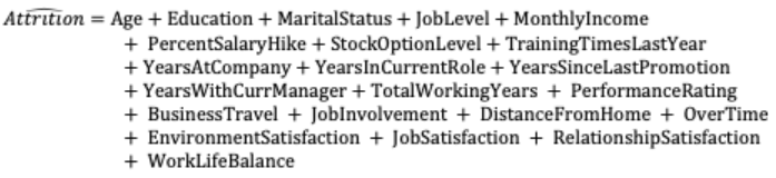
Using our intuition, we chose variables that made sense. Above is a list of all such variables. Using this model, we got an AIC of 966.81. To our surprise, most of the variables showed high significance with respect to Attrition except Education, Marital Status, Monthly Rate, % Salary Hike & Years At Company.

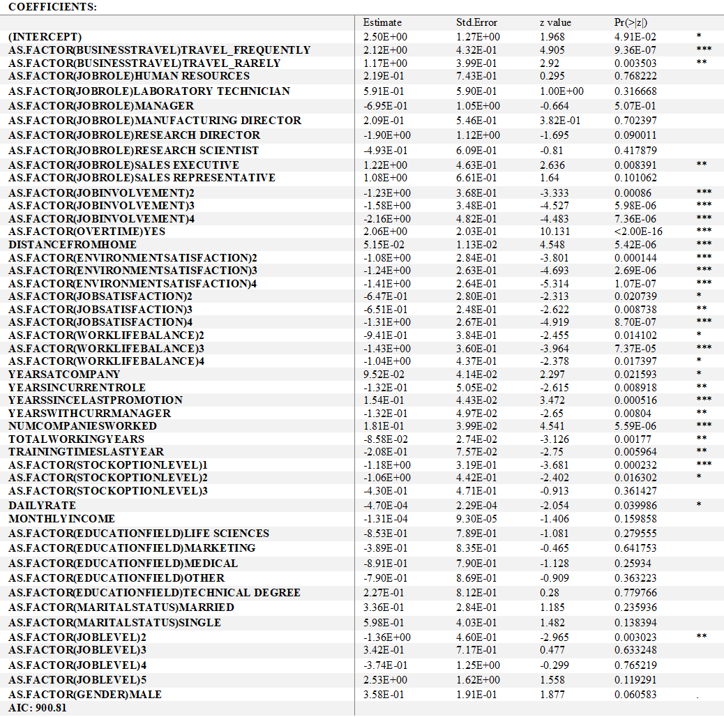
The Final Model

The model below combines all the significant independent variables from all the six categories. The results we got are not that shocking as columns like Job Involvement, Overtime, Distance from home made the cut and are highly significant. The approach we used seems to have done the job pretty as we were able to bring down a total of 34 variables to 22 variables. A majority of these variables are negatively correlated negatively with our target variable, Attrition. It means the higher these variables get in magnitude, the lower is the chance of Attrition (given everything else is held constant). The final AIC comes out to be 900.81.

6. Evaluation

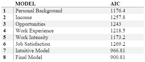
In the end, we have come up with eight models with different AIC’s. The model with the lowest AIC is indeed the one which we built using the most significant variables out of the original six categories. The most significant variables in this model are the one which actually matter when we talk about Attrition; these are :

1. Job Involvement

2. Over Time

3. Distance From Home

4. Environment Satisfaction

5. Years Since Last Promotion

6. Number of Companies Worked

7. Deployment & Future Scope

By selecting the above mentioned variables, we can determine whether a particular employee would leave the company or not. We believe our model can help organizations save millions of dollars in conducting training and workshops for new employees. Our model might still employ biases which have to be kept in mind while deploying the model. The future scope of our project can include playing around with the interactions of all the significant variables. That way, we might be able to improve the AIC score even more (bring it lower).

Tweet Share