Segmentation and Default Prediction of Credit Card holders
- 13 mins1. Introduction & Business Understanding
Since 1990 the Taiwanese government allowed the formation of new bank. Those banks turned their business largely on credit card business. They spent a lot of money on commercials and encouraged people to apply for credit cards to consume. In order to attract more customers, the banks lowered the requirements for credit card application. With the increase number of credit cards issued, accumulation of credit card debt started to grow into a big crisis for Taiwan. In February 2006 the total credit card debt in Taiwan reached to 268 billion USD1, 700,0002 people have become credit card-slaves, and their average money owed was 12,000 USD.
To decrease this kind of risk, once a credit card was issued to a customer, the bank needs to closely monitors the repayment ability of the customer. If there is a red flag rising in the customer’s credit card usage or reparent history, the bank needs to take action to lower the credit limit, increase APR or even suspend the credit card to manage the risk. For banks to be successful, our team capture the red flag signal using predictive modeling. During the sample period where we get our data from, our task is to identify high risk customers and taking the appropriate actions to prevent default in the next month and create further loss to the bank.
Our team gathered credit card payment history and default data from a Taiwanese bank for the year of 2005. Through this project, we’ll first try do customer segmentation by clustering users into different categories based on their demographic characteristics. Then we aim to determine the most important factors that affect defaulting in each category using various Machine Learning methods, thereby helping to predict whether a credit card holder would pay his/her impending monthly outstanding balance or not. The project comes under predictive analytics used in banking industry to avoid large possible defaults.
2. Data Description
There are 30,000 observations and 25 variables
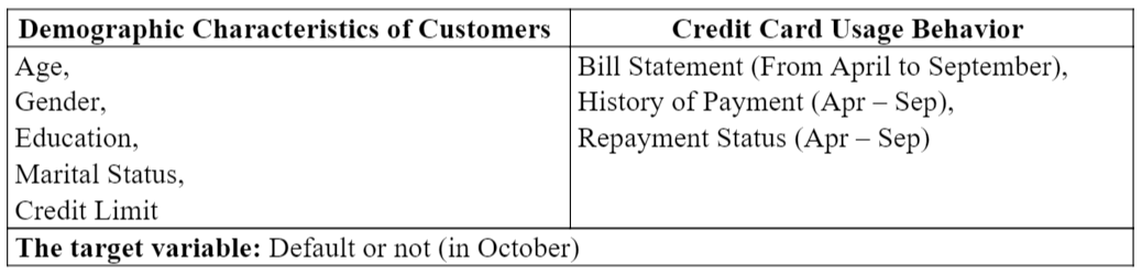
We divided the variables into two categories:
Credit limit is decided by the bank based on many factors, usually including the income of the customer. So, we include it in the demographic characteristics.
PAY_AMT in this data set is the amount of payment made in current month for the previous month. For example, amount of bill statement in July is corresponding to the payment made in August (e.g. BILL_AMT3 ~ PAY_AMT2). Thus, our specific definition of the target variable is whether the customer pay any amount in the October for the bill statement in September.
The columns names are generic in nature because once we build model, it can be scaled to determine whether an individual will default or not in a given based on the previous six-month payment history.
3. Data Preparation
The first step is to find missing values in the dataset. After running the MICE package, we find that there are no missing value in the data set. “ID” column doesn’t provide any information of the customer, so we drop it first. Then for better understanding, we change the names of bill amount and payment amount columns originally using number index to month abbreviation (e.g. BILL_AMT3 –> Bill_Amt_Jul). Also to better understand monetary terms, we convert the NT dollar to USD using exchange rate 1USD = 31.25NT Dollars (prevalent in 2005). Besides, to have a more realistic comprehension of the number, we could use the monthly cost of living in Taiwan in 2005 as a benchmark, which is 894 USD per household3.
4. Exploratory Data Analysis
As a first step, we wanted to ascertain whether people went overboard their respective limit balance, and if yes then how many. After running the appropriate query, we find 3931 entries out of 30000 who went overboard their allowable credit limit. So approximately, every 1 in 8 customers in our dataset exceeded the credit limit.
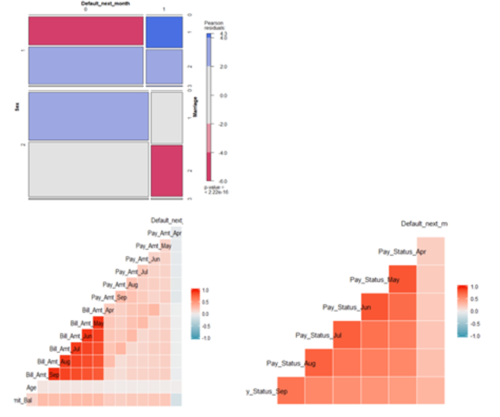
Next, we explored the correlation among variables. We draw correlation plots for continuous variables and categorical variables respectively. There exists significant correlation within bill statements and payment status for each month. Since our target variable here is binary variable, to examine its correlation with categorical variables, we also draw mosaic plot to see the correlation between demographical variables and default.
The colors in mosaic plot represent the level of the residual for that cell / combination of levels. More specifically, blue means there are more observations in that cell than would be expected under the null model (independence). Red means there are fewer observations than would have been expected. Here, the null model assumes that the default is independent from
marital status and sex. According to the mosaic plot, the default among married males exceeds the expectation of null model, while the default of married females is below the expectation. Besides, the non-default behaviors among married males are also significantly below expectation.
5. Customer Segmentation
Lending market is a huge one consisting of many types of customers. Every individual is different for a bank, on the basis of which the bank sets a limit balance. Example – a high earning individual is expected to enjoy the luxury of high credit balance, while a low earning individual may not be so lucky. Everything depends on the expected risk and propensity of the bank to take on risks.
That is why, we thought about segmenting the customers into different categories so as to provide a richer context while running models and providing recommendations. Steps followed for clustering –
Selecting and Standardizing customer demographic information
Out of the initial 24 variables, we selected just the 5 demographic variables such as Age, Gender, Education, Marital Status and Credit limit to form clusters. Out of them, Age and Credit Limit are continuous in nature so we scaled these columns down to values having standard deviation as 1 and mean as 0. The categorical variables such as Gender, Education and Marital Status were not scaled as each of them are in similar scale already and didn’t showcase large variance.
Knowing and Setting the optimum value of number of clusters
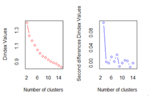
Being unaware about the bigger picture showcased by the dataset, we had to take help from external libraries such as ‘NbClust’ to come up with optimal number of clusters that could be successfully made from the dataset. We used ‘Elbow Method’ to find the optimal value of 3 as our intended number of clusters. Our dataset consists of 30k rows which makes it time and hardware consuming process to complete. As a result, we scaled it down to 1000 samples on which we ran the test.
As per the second graph shown above, the highest drop in dindex value occurs while transitioning from 2 clusters to 3 clusters. Therefore, we concluded that 3 is the optimum number of clusters.
Applying K-means clustering
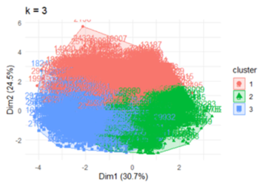
After finding out 3 as the optimal value, we made use of ‘kmeans’ library to differentiate each record into one out of three clusters. As a result, we were able to divide each customer on the basis of his/her demographic information.
Identifying characteristics of each cluster
Finally, it was time to run Exploratory Data Analysis on each cluster to find the peculiar behavior showcased. After running the analysis, we came up with this differentiation
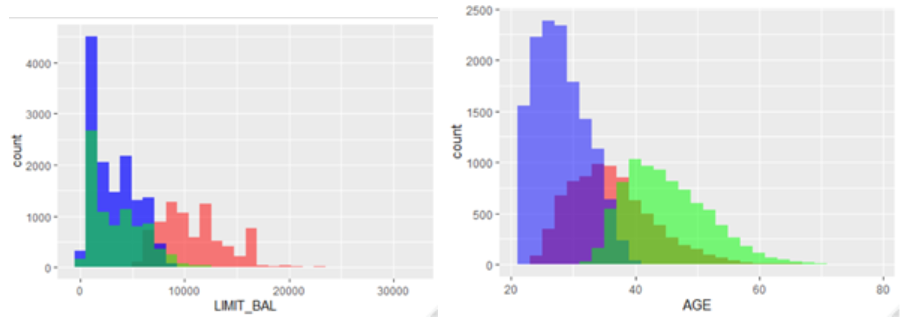
A) Cluster 1 (Red in color): 7962 records.
The limit balance in this cluster typically stood in the range of $5k to $20k. Also, the customers are middle aged in this cluster.
B) Cluster 2 (Blue in color): 13767 records.
The limit balance in this cluster typically stood in the range of $0 to $8k. Also, the customers are young in this cluster.
C) Cluster 3 (Green in color): 8271 records.
The limit balance in this cluster typically stood in the range of $0 to $12k. Also, the customers are bit on the older spectrum in this cluster.
6. Modeling
After differentiating customers into different clusters according to their limit balance and age, we move on to the modeling part. The dataset is first differentiated according to the three clusters mentioned above, then each cluster was divided into training and testing components (with 75% converted to training set and the rest designated as test set). As this is a binary outcome problem, we applied the Stepwise Logistic Regression, Random Forest and Lasso Regression, and then chose the one showing the most promising variance and bias.
Stepwise Logistic Regression
Under this method, AIC of all combinations of possible regressors is computed and the combination showcasing the lowest AIC is chosen. It is essentially a simple regression model with an added advantage of stepwise selection that manually calculates AIC of all combinations of possible regressors and selects the one with smallest AIC. For each cluster, we get different set of variables that are significant for that particular cluster. For example: in cluster 1, the amount payed in previous month, such as Limit Balance, are important. While in cluster 2, sex of the customer and payment made three months back are important.
Random Forest
For node size, we choose 1 to achieve best accuracy. For number of trees, we decided it based on inequality: ntree × node size>number of observations . For number of variables available for splitting at each tree node, we use the default value, which is the square root of the number of predicator variable. In all three clusters, the most important variables are the payment status and bill amount in September.
Lasso
In order to control the complexity of the predictive model, we use LASSO to determine the optimal penalization parameter λ. We included all the interactions and applied three rules, including the minimum of the mean values, 1se to the right and the theoretical valid choice, to compute Lasso for all values of λ. Then we used cross validation and showed the whole path to pick the λ. For each cluster, the λ is 16, 12, 23 respectively. The selected variables in Cluster 1 include Pay_Sept, Pay_Aug, Pay_July, Limit_Bal:Education. The selected variables in Cluster 2 include Pay_Sept, Pay_Amt_Sep, Pay_Sept:Pay_Aug, Pay_Sept:Bill_Amt_Sep. The selected variables in Cluster 3 include Pay_Sept, Pay_Aug, Pay_July, Pay_May.
7. Model Evaluation
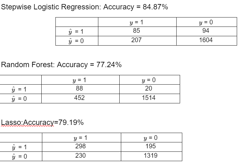
We chose the threshold at 0.3 because of the heavy loss the bank will incur if False Negative rate is high. So, choosing 0.3 is conventional enough to get a low False Negative rate as well as ambitious enough to maintain good accuracy.
Stepwise Logistic Regression: Accuracy = 84.87%
Random Forest: Accuracy = 77.24%
Lasso:Accuracy=79.19%
Based on the out-of-sample accuracy (cluster2: log-79.4%, lasso-86.16%, rf-86.14%; cluster 3: log-77.6%, lasso-77%, rf-86.48%), we choose Logistic for the customers who belongs to cluster 1, Lasso for cluster 2, and Random forest for cluster 3.
8. Deployment
Our end goal is to maximize Bank’s profit (or minimize loss) for which, the False Negative percentage should be as low as possible along with overall accuracy as high as possible. Therefore, the threshold used to classify should take care of these factors so as to create a perfect mix of accuracy and business value. Considering every factor, the stepwise logistic regression performed the best out of all the models in cluster 1. Due to time and computational constraints, we couldn’t complete tests on clusters 2 and 3 but as a future scope, we can definitely work on them.
9. From Predictive Modeling to Risk Management
Once a credit card was issued to a customer, the bank need to closely monitor the repayment ability of the customer. If there is a red flag rising in the customer’s credit card usage or reparent history, the bank needs to take action to lower the credit limit, increase APR or even suspend the credit card to manage the risk. For banks to be successful, our team capture the red flag signal using predictive modeling. During the sample period where we get our data from, the major challenge is to identify high risk customers and taking the appropriate actions to prevent default in the next month and create further loss to the bank.
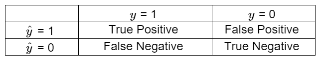
Decisions based on Classification :
The Expected value of decisions:
X: Customer info, A: Suspend credit card
| E [loss | X, A] = P (TP | X, A) * (Value - Cost) + P (FP | X, A) * (probability of customer leaving * APR) |
True Positive:
In our case true positive means we successfully predict the customer would default in the next month and the customer did default.
Action & Value: For customers we predict will default in the next month, we advise the bank to suspend this customer’s credit card. Implementing our strategy could send a warning signal to the customer who would default and prevent those customers accumulates even higher credit card debt in the following month. Moreover, our strategy helps banks contain the risk of eventually have to write off the customer and lost all the money.
False Positive:
In our case false positive means we predict the customer will default in the next month but the customer is able to repay the bill.
Action & Risk: The bank will still suspend the customer’s credit card. However, in reality the customer has the finical capability to repay the bill. Therefor the customer might feel unsatisfied with bank’s service and might switch to another bank’s credit card service.
False Negative:
In our case false positive means we predict the customer would not default, but in the next month the customer did default.
Action & Risk: Since we did not successfully predict the customer would default, the bank would not take any action toward to the customer. Therefore, the customer is allowed continue to use the credit in the next month which will accumulate more debt and the chance of the customer would default again also increases.
True Negative:
We successfully predict the customer would not default in the next month, and the customer did not default.
Action & Risk: No addition value added.

Archit Gupta
An analytical being in this not so analytical world